
|
In the last issue of the CSA Newsletter there was an article concerning the use of CAD in the excavation at Nemi, Loc. Santa Maria, and there was also a promise of more information about the use of computers at that site. In this article we will describe the construction and implementation of a database model for the registration of finds and their context in the Nemi excavation. This also involves a method to compute the volume of a convex soil block based on the three-dimensional coordinates of its vertices and then to compute the density of the different categories of finds in every soil block. This enables us to add quantitative figures to the different soil blocks throughout the site and makes it possible to automate comparing soil blocks.
Our intention was to create a data model to organize and relate all documentation about the finds and their contexts. The basic unit for the context we call a "soil block." Soil blocks are intended to represent smaller units than the archaeological layers identified by the excavators. The soil block is also the basic unit in the database. For each soil block information is recorded, i.e. soil description, contents of organic material, stones etc. Furthermore, the method of digging is recorded as an indication of the quantitative recovery of finds, i.e., if the soil block has been dug with a diesel-powered mechanical excavator, the recovery of finds is not as good as when trowel and sieve have been used. The description is divided into different fields to ease database queries.
Each soil block has an identification code (SB_ID): a unique combination of: first two letters assigned to the the trench; then two figures for the layer, as recognized by the excavators; and finally two figures for the soil block in that layer. We will later return to the registration of the absolute position of the soil block in detail, but it consists of a list of three-dimensional coordinates. Each set of coordinates is given a reference number and, together with the SB_ID, it forms a combined key.
Fig. 1: Database diagram showing the different tables and their relationships to one another.
After the finds - ceramics, metal objects, building materials etc. - have been washed, they are grouped in different categories, where the pottery of course is subdivided into the various groups represented at the site. All sherds are then counted and weighted, and diagnostic pieces are sorted out for individual numbering, description, drawing, and photography. This creates two more tables for the database. One for the total finds from one soil block, where the SB_ID and the ware group is a combined key and another table with the catalogue description for the individual finds. Here the find number is the key, and the SB_ID a foreign key that enables us to link the individual finds to their context.
The context and finds are by now registered and linked, but without any references to the graphic documentation, i.e., photos. As with everything else, each photo has its own unique number and information, such as: film type (i.e., 6 X 6, black and white), date, time, etc. But since the individual photo can include many finds, we need a list for each photo with the keys for the photographed objects, which in this case are the find numbers. However one find can also be photographed many times. Therefore, this list has to work both ways since this table can be approached either from the find catalogue or from the photo list. The key for the reference list is made as a combined key, with the photo number and the foreign key.
Usually coordinates of the vertices are used as part of the description of the position of the soil block, but this information is not generally sufficient. Rather than requiring further information - like specifying the relation between the vertices by coding or graphically (Fig. 2 B and C) - we decided to require the soil block to be treated as a convex polyhedron. Similar to a polygon, which is a two-dimensional object defined by a number of lines, a polyhedron is a three dimensional object defined by a number of planes constituting the surface of the polyhedron. A polyhedron is convex if for any two points in the polyhedron, the line connecting them lies completely within (or on the surface of) the polyhedron. This means that the polyhedron has no cavities, i.e., if one imagines pulling a rubber balloon around the polyhedron, it would fit tightly to the surface of the polyhedron everywhere. Excavating the soil blocks according to this has proven to be easy; however the output of only coordinates has been difficult for some to keep track of, so they have had to draw sketches of the soil blocks to feel confident of their measurements.
Fig. 2: A two-dimensional example of uncertainty when a set of points, A, does not supply sufficient information to determine the shape of the object, since the points can be related as in B or C. For this particular set of co-ordinates no convex polygon can be constructed with all the points as a vertices.
Given the set of points (the coordinates of the vertices of the soil block), we determine the convex hull of these points, that is, the smallest convex polyhedron containing all the points. This convex hull is defined as a group of triangular surfaces covering the hull and together making its full surface, as in Fig. 3.
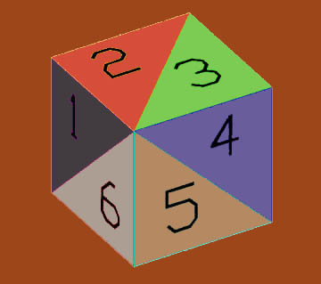
Fig. 3: A sample triangulation of an object's surface from a single vertex, in this case of a cube. Only the triangulations of the visible surfaces can be seen.
By joining these triangular surfaces to the one of the vertices (in Fig. 4 the visible triangular surfaces from Fig. 3 are shown as joined to the only vertex not visible in Fig. 3, i.e., the lower back corner), the convex hull is now defined by a number of joined tetrahedra (a polyhedron defined by four triangular surfaces). When this process is performed automatically, a number of additional tetrahedra are also formed, all with zero depth and, consequently zero volume. They are not shown in the drawings.
 |
 |
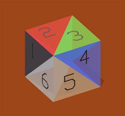
| Fig. 4 - The cube illustrated in Fig. 3 but shown as a group of translucent tetrahedra. | Fig. 5 - The tetrahedra in Fig. 4 shown separated to illustrate their individual shapes. |
The reason for maintaining the convex hull this way is that for an arbitrary, convex polyhedron there is no simple formula for calculating the volume of the polyhedron. But for any tetrahedron the volume can be calculated from the coordinates of the vertices, cf. e.g. Fraleigh and Beauregard, page 203. Then the volume of the polyhedron can be calculated as the sum of the joined tetrahedra forming the convex hull. Since the number of vertices in the soil blocks is not very high, rarely exceeding ten, we have used a simple algorithm, where the time used for calculation rises with the square of the number of vertices, to determine the triangulation of our convex soil blocks. This algorithm is described in de Berg, van Kreveld, Overmars, and Schwarzkopf, chapter 11. We have implemented the algorithm to accomplish the tasks in JAVA and the resulting program, which also checks for some possible errors in the measuring, calculation, and filing of coordinates, has been used during the last two campaigns. The JAVA source code is available on request.
With a three-dimensional digital registration of the finds and the volume of the soil block, the density of the different find categories in the soil block, either by weight or number, is easy to determine. A center coordinate for the soil block is also necessary for illustrating the soil block graphically and selecting it for database queries. The center coordinate is calculated by averaging the X, Y and Z coordinates for all the vertices of the soil block. For a convex soil block, this gives a point within the soil block, which is sufficient for our purposes.
From these data we are able to reconstruct our excavation. The data can be retrieved from the database in pre-designed tables, and in this way the database works like an old-fashioned archive where the information is written on catalogue cards. But it may not give us a clear impression of what we have excavated yet. To obtain further insight we need to analyze our data, to find patterns among the finds, their contexts, and how these relate to the different structures. This is where we reap the full benefit of the digital registration, as it provides ample opportunity for combining the data and visualizing the result graphically. We are able to see patterns in an otherwise misty pile of numbers.
We illustrate this by the following example of use of graphical presentations of database queries. The Trench N was excavated during the 1999 campaign and laid out north/south to give a date for the wall in the southern end, a wall that forms the back wall in a larger building complex. Seventy soil blocks were excavated with a total of 2186 finds registered. In the northern end of the trench some almost horizontal layers were excavated. To get started analyzing the trench, we examined the distribution of the density of the different finds categories in these layers, i.e., in soil blocks north of our 5018.50 mark. The result was plotted in an MS-Excel diagram, relating the different finds categories to their levels (see Fig. 6).
 .
.
Fig. 6: The relation of different finds categories and their levels.
It is here easy to see, that around level 330.75 remarkable changes occur in the density of mainly building materials and also in what has been diagnosed as amphorae and plain ware. Below level 330.25 mainly impasto (Iron Age) pottery was found. Without even looking at the dating of the specific sherds we have thus identified 3 layers (plus the plow soil at the top containing post-antique material) in the northern part of the trench. To see how these layers are distributed over the entire trench, all soil blocks that fulfill a requirement of high concentrations of the different categories of building material, amphorae, cooking ware, etc. are plotted as a projection on the profile drawing (Fig. 7).
Fig. 7: A projection of the soil blocks on the profile drawing where the small blue squares show all soil blocks. North is to the right, and the soil blocks used for Fig. 6 are those to the north of the vertical blue line indicating the 5018.5 mark.
The blue squares do not reflect the differing sizes of the soil blocks, making their distribution appear to be uneven.
The soil blocks with larger blue boxes around them contained only impasto and the ones with red boxes had a high concentration of building material. The soil block designated by the red arrow contains probably a miss-diagnosed sherd, since it is positioned in the middle of an otherwise clean Iron Age layer.
This identifies the foundation trench, the Roman layer without much building material and the Iron Age layer.
Before accepting the layer separations derived from the finds densities, one must be sure that the decrease in the density of building material was not caused by a different method of digging or recovery. This information is readily available in the soil block descriptions. It is however unlikely that this decrease can be explained by anything but a layer change.
During the first three excavation campaigns computers, databases, and total stations have become a natural part of the fieldwork. Already by now this has allowed us to benefit from an efficient and easily accessible archive. We believe that this archive and the quantitative methods for analysis it facilitates will also prove useful during the publication phase. A further step in the treatment of our data would be to apply statistical methods to the material. The detailed and organized registration provides a firm foundation for statistical analyses that will yield further conclusions.
[1] M. de Berg, M. van Kreveld, M. Overmars, and O. Schwarzkopf. Computational Geometry, Algorithms and Applications. Springer-Verlag, Berlin, Germany, 1997
[2] J. B. Fraleigh and R. A. Beauregard. Linear Algebra. Addison-Wesley Publishing Company, Reading, Massachusetts, U.S.A., 1990
Søren Fredslund Andersen, Department of Classical Archaeology, University of Aarhus
Rune Bang Lyngsø, University of California at Santa Cruz, School of Engineering
To send comments or questions to either author, please see our email contacts page.
For other Newsletter articles concerning the use and design of databases, Electronic Publishing; or the use of electronic media in the humanities; consult the Subject index.
Next Article: Inheriting a Poor Database
Table of Contents for the Fall, 2000 issue of the CSA Newsletter (Vol. XIII, no. 2)
 Table of Contents for all CSA Newsletter issues on the Web