
| Vol. XXVI, No. 1April, 2013 |
Articles in Vol. XXVI, No. 1
Digital Data — Ur of the Chaldees: A Virtual Vision of Woolley's Excavations
Preserving data from a very old excavation
-- William B. Hafford
Rethinking CAD Data Structures — Pompeii Archaeological Research Project: Porta Stabia
Making AutoCAD easier to use effectively
-- Gregory Tucker, University of Michigan, and John Wallrodt, University of Cincinnati
Website Review: Penn Museum
An enormous website with more pluses than minuses.
-- Andrea Vianello
How Often Must We Reinvent the Wheel?
Where do students go to learn about digital technologies?
-- Harrison Eiteljorg, II
Data in the Future — Archived or Locked?
Prison terms for data retrieval?
-- Harrison Eiteljorg, II
Miscellaneous News Items
An irregular feature
To comment on an article, please email
the editor using editor as the user-
name, csanet.org as the domain-name,
and the standard user@domain format.
Index of Web site and CD reviews from the Newsletter.
Limited subject index for Newsletter articles.
Direct links for articles concerning:
- the ADAP and digital archiving
- CAD modeling in archaeology and architectural history
- GIS in archaeology and architectural history
- the CSA archives
- electronic publishing
- use and design of databases
- the "CSA CAD Layer Naming Convention"
- Pompeii
- pottery profiles and capacity calculations
- The CSA Propylaea Project
- CSA/ADAP projects
- electronic media in the humanities
- Linux on the desktop
Search all newsletter articles.
(Using Google® advanced search
page with CSA Newsletter limit
already set.)
Rethinking CAD Data Structures — Pompeii Archaeological Research Project: Porta Stabia
Gregory Tucker, University of Michigan, and John Wallrodt, University of Cincinnati
(See email contacts page for the author's email address.)
Since 2005 the Pompeii Archaeological Research Project: Porta Stabia (PARP:PS), directed by Steven J.R. Ellis at the University of Cincinnati, has studied the insulae at the southern end of the via Stabiana, near the Stabian Gate. (See classics.uc.edu/pompeii.) The project is refining the early history of this part of Pompeii and better defining its dynamic relationship with the development of the public spaces to its north and west. Identifying and defining the response of non-elite, working-class, families to the significant changes to socio-economic and political systems across the Mediterranean from the 4th century BC until the late 1st century AD has been a consistent priority. Through archival research, material analysis, geophysical survey, architectural survey, and excavation a new narrative has come to light about the role ancient Pompeiians played in shaping the ancient city, influenced by evolving relationships with far-flung provinces. (For a thorough list of PARP:PS publications, please visit classics.uc.edu/pompeii/index.php/reports/publications.html).
Work in the area around the Porta Stabia, first excavated in the 1870's, revealed architecture forming the walls of rooms and boundaries of properties. Thus, PARP:PS is excavating in what was a fully urban portion of Pompeii, and, as a consequence, the PARP:PS staff must work within spaces restricted by surviving elements of ancient structures. From 2005-2010 architectural survey and archaeological excavation focused on insula VIII.7, on the west side of the via Stabiana, crossing the street to insula I.1 in 2010. Entering the second year of excavations in insula I.1, in 2011, the team decided that the spatial data obtained through total station survey and archaeological drawing1 should be reorganized and placed into a planned, deliberate structure which could accommodate future data collection and be easily accessible during subsequent study seasons. This article outlines the structure that PARP:PS uses to manage spatial data within AutoCAD®.
The architecture still standing in these areas encourages documentation of spatial data using CAD software for its precise drafting capabilities. Using CAD software as the primary interface with the spatial data is standard practice in such conditions, especially considering the ease of transferring data between and among CAD, GIS, and other spatial software packages. From 2005-2010 AutoCAD was used to organize these data, and our documentation system grew organically as demands arose and new data were added. With the move across the via Stabiana to insula I.1 in 2010 a new AutoCAD model was developed, based on the same structure and naming conventions used for the VIII.7 data. One of the goals of the 2011 season was to revise the structure of the CAD model so that data were deliberately organized in a way that was easy to work with during field seasons, accessible to non-specialists during the rest of the season, and flexible enough to accommodate future revisions and additions.
The new data structure employed with the CAD model was intended to present as much information as possible with minimal reliance on external documentation or support. As with many of the digital data policies for PARP:PS, facilitating convenient access for all project members to the spatial data was a priority. The CAD model was expected to be used as a reference by project members in writing reports, generating plans, and contributing to other various outputs. One assumption made during the creation of the file-naming system was that anyone accessing the CAD model for these purposes would also have access to the project database, maintained in FileMaker®, which contains detailed information, interpretation, and analysis for the features and contexts that are represented in the model. Although there are no direct links between the Filemaker database and the AutoCAD model, the naming system being described here is clear enough that matching the records in the database with features in the model could take place quickly and seamlessly. The CAD model should therefore be a supplementary resource that any team member can use without the assistance of a specialist and in conjunction with the database to access more qualitative data.
The earlier system in place for the CAD model used common-language layer names. For example, layers had names such as "Wall Bases," "56000 Limits," or "56009" (56000 is the name of a trench, and 56009 is a stratigraphic unit — SU hereafter). The major advantage to the old system is that it was easily understood by team members without requiring familiarity with a coding system. Also, without a coding system and with many elements on each layer, it was easy to add or edit data in any layer without having to recognize the specific codes for that layer. These broader, more general terms had their use, but the desire for a more robust data structure necessitated the change in 2011 to the current system.
Whatever the new system was to look like, keeping each SU on its own individual layer was expected to result in hundreds of layers, making the entire layer list impractical to use due to its excessive length. In preparation for whatever conversion was to take place many common group filters (an AutoCAD term — a group filter is just a name for a batch of layers, permitting the entire batch to be called up via the group name alone) were created. Any individual layer could be assigned to multiple group filters. For example, the layer "56000_BaseLine" is in both the "2011_Trench_BaseLines" group and the "56000" group.
Given the project's use of CAD to document the site's spatial information and the desire for a thoughtful organization of the data within our model, we sought out methods and structures that were already proven successful, which lead to Eiteljorg's CSA Layer-Naming Convention approach and a modification of it discussed in a CSA Newsletter article in Vol. XXII, 2; September, 2009, by Eiteljorg and Paul Blomerus "Managing the Content of AutoCAD® Models with Layers,". Developed over more than twenty years and adapted to fit multiple goals, this system is a proven way to maximize the functionality offered by AutoCAD and to provide a tremendous amount of metadata about individual elements through the layer names alone. This approach, and the adaptation developed by Blomerus and Lesk ["Using AutoCAD® to Construct a 4D Block-by-Block Model of the Erechtheion on the Akropolis at Athens, III: An interactive virtual-reality database" XXII, 1 (Spring, 2009)], were designed for projects documenting large architectural structures on the Athenian Acropolis. Eiteljorg provided suggestions for adapting this system for models of active excavations using similar principles, naming layers by year, trench, SU, and analytical codes, including time periods.
The basic framework of the CSA Convention rests on the use of codes and abbreviations which allow for very detailed queries and filters of the data using wildcards and the advanced search features available in AutoCAD. These conventions would provide a tremendous amount of information to the knowledgeable user just from the layer names themselves, and would allow anyone familiar with the software to query the model quickly and easily for data related to their specific research questions. However, where the CSA system was developed to manage quantitative and qualitative spatial data after field work (and considerable analysis) had been completed, our system is intended to manage these data during active field work. This distinction, combined with the goal of maximizing ease of use by non-specialists and by those unfamiliar with wildcard characters and other filtering shortcuts within AutoCAD, made us consider potential alterations to the CSA system. Given the obvious benefits of the CSA Convention, we decided to attempt to adapt the system to work parallel to the FileMaker database, as opposed to duplicating information that team members would likely seek elsewhere in the first instance.
The goals of the PARP:PS naming convention were to be immediately recognizable and intuitive to new or occasional users while being simple and limited in the length of the layer names so as not to appear intimidating. With the move towards tablet computing by PARP:PS,2 the development of AutoCAD WS by AutoDesk for tablets, and the freely available student versions of AutoCAD for desktop computing, the model itself was accessible to the entire team at any time. Although the new naming convention would not increase the availability of the data, it was this ubiquitous availability that drove the push for a revision to the naming system. The resulting group filters and layer names are clear and accessible to anyone who is expected to access the model directly. Much of the information that Eiteljorg suggests to include in layer names for excavation is already included in the SU names. For instance, the SU titled "56009" already describes what year (56000 is from 2011), what trench (56000), and what SU (56009). Adding characters representing qualitative data about modeled elements would be superfluous prior to the completion of pending analyses; even when available such information will be housed in the FileMaker database.
The resulting system uses a series of prefixes to help with sorting, grouping, and searching through layers separated from more detailed information as to their content with an underscore ( _ ). This approach allows for a limited number of prefixes, as described below, with some common language appendages. For elements that are coded with discrete identifiers in other documentation, such as the database, the same identifier is preserved for the spatial data. For instance, stratigraphic units and wall segments are identified with their respective prefixes plus the underscore and the numbers assigned in the field. Other elements are given clear common language identifiers, such as threshold data being assigned to the "FE_Thresholds" layer. The list of layer prefixes currently in use by PARP:PS is outlined below, and an example of a set of layers can be found in Figure 1.
Layer Prefixes
- FE_ (Features) These include doorways, stones, thresholds, and wall plaster.
- I2_ (Insula I.2) Data from insula I.2.
- PL_ (Plans) The baseplan for insula I.1, includes a schematic of the Soprintendenza plan and the plan for the Porta Stabia.
- PY_ (Past Years) Leftover layers and stray features that are not identifiable nor documented. They are preserved here rather than being deleted.
- SA_ (Soprintendenza Archeologici) Data provided by the Soprintendenza Speciale per i Beni Archaeologici di Napoli e Pompei. The SA_ plans are the detailed Soprintendenza plans for all of Pompeii, including plumbing, electrical cables, site boundaries, etc.
- SU_ (Stratigraphic Units) The limits and topographical survey data for the SUs for insula I.1, prior to excavation. These are further assigned suffixes when more information is necessary, such as when the same SU is recorded in a drawn plan and in a total station survey. Then the layer names holding these different data are appended with "p" or "ts," as appropriate.
- TR_ (Trenches) Information regarding the trenches, such as limits and baselines.
- UP_ (Utility - Points) The survey points are contained on these layers, specified by survey job title.
- UT_ (Utility - Trenches) Layers defining excavation information, especially labels, such as room numbers or trench names.
- WF_ (Wall Faces) Labels for the wall faces.3
- WS_ (Wall Segments) Individual wall segments on separate layers, with their labels on another layer.
- WW_ (Walls) These are the surveyed wall bases, tops, and verticals.
- WX_ (Excavated Walls) The excavated extensions of wall bases and verticals.
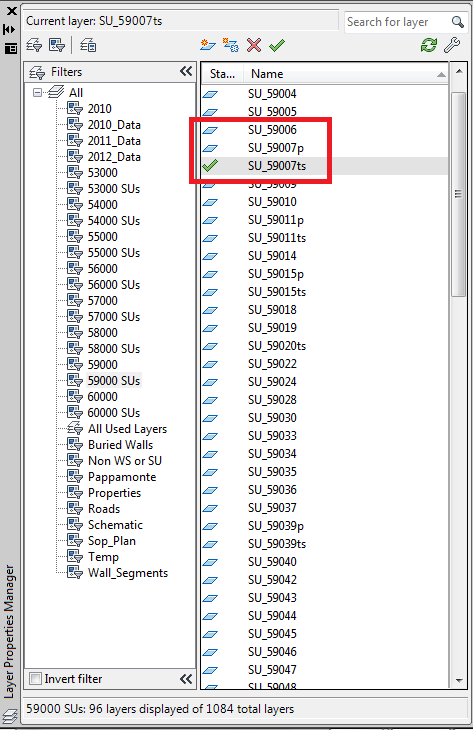
Fig. 1 - Example of layer list with prefixes. Note that there are
currently 1084 layers making using the entire list quite cumbersome.
The majority of the 1084 layers currently active in the CAD model represent excavated SUs, and an example of how they appear in the list can be seen in Figure 1. Highlighted in the red box are three SUs which are parsed out here:
- SU_59006 — "SU", indicates that this layer represents a Stratigaphic Unit; "_", is a spacing character between the layer type identifyer and the more detailed information; "59006", is the Stratigraphic Unit modeled on this layer ("59" indicates trench 59, and the "006" indicates the sixth SU from that trench).
- SU_59007p — As above for SU_59006, with the addition of "p" to indicate that the features on this layer were drawn by hand. This is only appended when an SU is drawn both by hand and by total station.
- SU_59007ts — As above for SU_59006, with the addition of "ts" to indicate that the features on this layer were drawn with total station data. This is only appended when an SU is drawn both by hand and by total station.
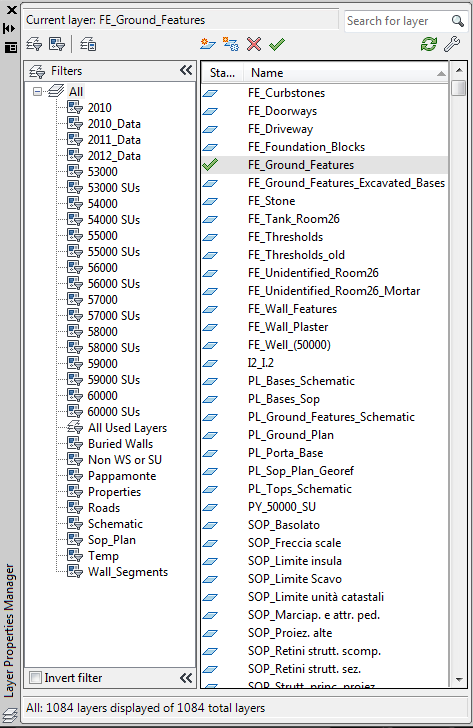
Fig. 2 - Example of layer list with prefixes.
The group filters defined in the model attempt both to group similar elements and to isolate them from the remainder of the model. A group filter might include only SUs interpreted as buried walls, for instance. Using them makes navigating the layer list simpler. A complete list of the current filters, which are added to and revised by the specialist in dialogue with those who are writing the excavation reports, is outlined below:
Filters
- 2010 — Contains all of the layers that originated in 2010, whether they were modeled in 2010 or 2011.
- 2010_Data — Contains the layers with the 2010 survey points.
- 2011_Data — Contains the layers with the 2011 survey points.
- 2012_Data — Contains the layers with the 2012 survey points.
- 53000 [- 60000] — Contains the baselines, limits, targets, and names for the respective trench.
- 53000 [- 60000] SUs — Contains the plan drawings and survey results from the 2011 trenches.
- Buried Walls — Contains the SUs interpreted as buried walls.
- Non WS or SU — Contains all of the layers not beginning with SU or WS (these excluded layers make up the vast majority of the total number of layers and viewing/manipulating the remaining layers is easier when they are excluded from the list).
- Pappamonte — Contains the SUs representing an early type of stone used in Pompeiian construction, pappamonte.
- Properties — Contains the UT layers which outline the individual properties identified in insula I.1.
- Roads — Contains the SUs representing roads.
- Schematic — Contains the SUs that could be useful as a baseplan or schematic plan of the insula.
- SOP_Plan — Contains the layers beginning with SA_, to isolate the data that the Soprintendenza has available.
- Temp — Contains layers that are part of active data processing routines by the technician, but are otherwise not intended to be part of a permanent group useful to other users.
- Wall_Segments — Contains all of the wall segments.
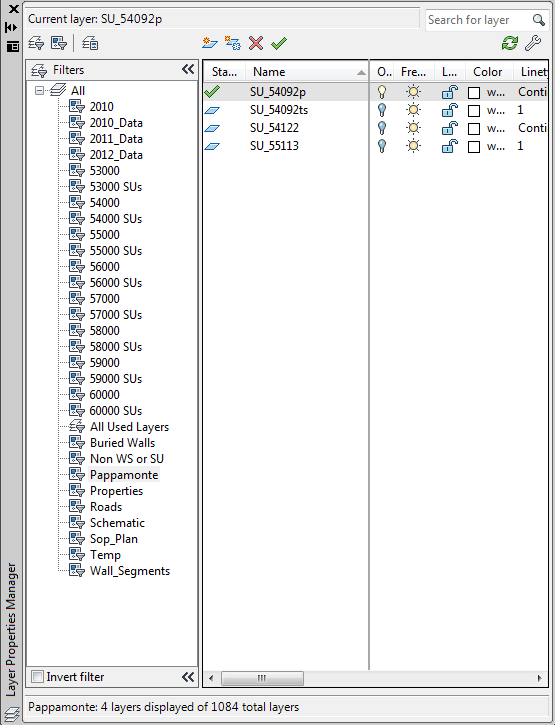
Fig. 3 - Example of the group filters in use. In this case the “Pappamonte”
filter is selected and all four SUs currently modeled that have been
identified as pappamonte blocks are displayed, with only the first,
and current, layer (SU_54092p) active for this example.
Much like PARP:PS itself, the CAD model is a work in progress, which is constantly improving and evolving. Looking back at the data from the first nine years of the project, covering insula VIII.7, and adapting these layers to the current system is a goal for the upcoming year, and there does not appear to be any reason why this process should be difficult or cumbersome, given the ease of converting the insula I.1 data. As more stratigraphic units are dated and identified as significant moments or representative of patterns between excavation areas, filters will likely be added for time periods or phases. Additionally, there will likely be prefixes that must be added, but this is as simple as developing another two character prefix to assign to the new layers. For the past two years there have been no unforeseen prefixes added, while the filtered list has grown as more analytical groupings have been requested. With these filters an alternative is provided to the coding and search methodology suggested by Eiteljorg in the CSA Convention.
Applying the concepts developed in the CSA Convention and adapted elsewhere has resulted in a data management strategy that we believe is accessible to non-specialists while remaining robust enough to group, sort, or identify elements and features of desired qualities. As more straticgraphic units and standing architectural elements are documented, they can be added to the model and their layers sorted into the appropriate filters. The PARP:PS system could be easily adapted and applied to any in-progress excavation and will allow us to make a potential transition to a more thorough naming system easily when each wall and unit has been completely analyzed after the completion of the project’s active field work.
-- Gregory Tucker and John Wallrodt
Notes:
1. For more information on the drawing process please see the following posts from the Paperless Archaeology Blog: paperlessarchaeology.com/2011/07/10/11-drawings-workflow/ and paperlessarchaeology.com/field-drawings/. Return to text.
2. See, for instance, the presentations by the PARP:PS team at the Computer Applications and Quantitative Methods in Archaeology (CAA) meetings in Beijing (2011), Southampton (2012), and Perth (2013). Return to text.
3. The architectural analysis methodology that leads to divisions based on faces, segments, and other categorization is discussed in S. Ellis, T. Gregory, E. Poehler, and K. Cole 2008 "A New Method for Studying Architecture and Integrating Legacy Data: A case study from Isthmia, Greece," Internet Archaeology 24, at intarch.ac.uk/journal/issue24/ellisetal_index.html. Return to text.
All articles in the CSA Newsletter are reviewed by the staff. All are published with no intention of future change(s) and are maintained at the CSA website. Changes (other than corrections of typos or similar errors) will rarely be made after publication. If any such change is made, it will be made so as to permit both the original text and the change to be determined.
Comments concerning articles are welcome, and comments, questions, concerns, and author responses will be published in separate commentary pages, as noted on the Newsletter home page.